Basic Usage, small protein

`Gromacs_py` basic example

Here is an example of a short simulation of the SH3 domain of phospholipase C$:nbsphinx-math:`gamma`$1. Five successive steps are used:

Topologie creation using GmxSys.prepare_top().
Minimisation of the structure using GmxSys.em_2_steps().
Solvation of the system using GmxSys.solvate_add_ions().
Equilibration of the system using GmxSys.em_equi_three_step_iter_error().
Production run using GmxSys.production().

Import

[1]:

import sys
import os
import urllib.request
import pandas as pd
import matplotlib
import matplotlib.pyplot as plt
import numpy as np
import seaborn as sns

To use gromacs_py in a project:

[2]:

from gromacs_py import gmx

Simulation setup

Define a few variables for you simulation, like:
- simulation output folders
- ionic concentration
- number of minimisation steps
- equilibration and production time

[3]:

DATA_OUT = 'data_sim'
PDB_ID = '1Y0M'

# System Setup
vsite='none'
ion_C = 0.15
sys_top_folder = os.path.join(DATA_OUT, 'sys_top')

# Energy Minimisation
em_folder = os.path.join(DATA_OUT, 'em')
em_sys_folder = os.path.join(DATA_OUT, 'sys_em')
em_step_number = 5000

# Equillibration
equi_folder = os.path.join(DATA_OUT, 'sys_equi')
HA_time = 0.5
CA_time = 1.0
CA_LOW_time = 2.0

dt_HA = 0.001
dt = 0.002

HA_step = 1000 * HA_time / dt_HA
CA_step = 1000 * CA_time / dt
CA_LOW_step = 1000 * CA_LOW_time / dt

# Production
prod_folder = os.path.join(DATA_OUT, 'sys_prod')
prod_time = 10.0

prod_step = 1000 * prod_time / dt

Get PDB file from the `rcsb.org` website

[4]:

os.makedirs(DATA_OUT, exist_ok = True)

raw_pdb = urllib.request.urlretrieve('http://files.rcsb.org/download/{}.pdb'.format(PDB_ID),
                           '{}/{}.pdb'.format(DATA_OUT, PDB_ID))

Create the `GmxSys` object

[5]:

md_sys = gmx.GmxSys(name=PDB_ID, coor_file=raw_pdb[0])
md_sys.display()

name         : 1Y0M
coor_file    : data_sim/1Y0M.pdb
nt           : 0
ntmpi        : 0
sys_history  : 0

Create topology:

Topologie creation involves: - protonation calculation using pdb2pqr and propka - topologie creation using pdb2gmx

[6]:

md_sys.prepare_top(out_folder=os.path.join(DATA_OUT, 'prot_top'), vsite=vsite, ff='amber99sb-ildn')
md_sys.create_box(dist=1.0, box_type="dodecahedron", check_file_out=True)

3D coordinates vizualisation using `nglview`

Use the view_coor() function of the GmxSys object to vizualise the protein coordinates.

Note that nglview library need to be installed :

conda install nglview

You’ll probably need to restart you notebook after installation to enable nglview widget appearance.

[7]:

view = md_sys.view_coor()
view.add_representation(repr_type='licorice', selection='protein')
view

[9]:

# Unecessary, only need to nglview online:
IFrame(src='../_static/1Y0M.html', width=800, height=300)

[9]:

Energy minimisation

[12]:

md_sys.em_2_steps(out_folder=em_folder,
                  no_constr_nsteps=em_step_number,
                  constr_nsteps=em_step_number,
                  posres="",
                  create_box_flag=False,
                  emtol=0.1, nstxout=100)

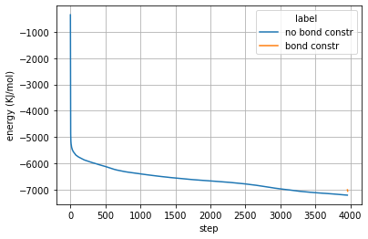
Plot energy:

[30]:

ener_pd_1 = md_sys.sys_history[-1].get_ener(selection_list=['Potential'])
ener_pd_2 = md_sys.get_ener(selection_list=['Potential'])

ener_pd_1['label'] = 'no bond constr'
ener_pd_2['label'] = 'bond constr'

ener_pd = pd.concat([ener_pd_1, ener_pd_2])

ener_pd['Time (ps)'] = np.arange(len(ener_pd))

gmx energy -f data_sim/em/Init_em_1Y0M.edr -o tmp_edr.xvg
gmx energy -f data_sim/em/1Y0M.edr -o tmp_edr.xvg

[31]:

ax = sns.lineplot(x="Time (ps)", y="Potential",
                  hue="label",
                  data=ener_pd)
ax.set_xlabel('step')
ax.set_ylabel('energy (KJ/mol)')
plt.grid()

../_images/notebook_00_basic_example_21_0.png

3D vizualisation using `nglview`

Not much append in the second minimisation, we can have a look at the first one using md_sys.sys_history[-1], which is considered as a GmxSys object.

Use the coor_traj atribute of the GmxSys object to vizualise the trajectory. Note that that the simpletraj library is a dependenie. To install simpletraj use:

pip install simpletraj

first you should make molecule whole using convert_trj() function.

[14]:

md_sys.sys_history[-1].convert_trj()

[75]:

view = md_sys.sys_history[-1].view_traj()
view.add_representation(repr_type='licorice', selection='protein')
view.center()
view

[77]:

# Unecessary, only need to nglview online:
IFrame(src='../_static/1Y0M_em_traj.html', width=800, height=300)

[77]:

Solvation (water and $Na^{+} Cl^{-}$)

[18]:

md_sys.solvate_add_ions(out_folder=sys_top_folder,
                        ion_C=ion_C)
md_sys.display()

name         : 1Y0M
sim_name     : 1Y0M
coor_file    : data_sim/sys_top/1Y0M_water_ion.gro
top_file     : data_sim/sys_top/1Y0M_water_ion.top
tpr          : data_sim/em/1Y0M.tpr
mdp          : data_sim/em/1Y0M.mdp
xtc          : data_sim/em/1Y0M.trr
edr          : data_sim/em/1Y0M.edr
log          : data_sim/em/1Y0M.log
nt           : 0
ntmpi        : 0
sys_history  : 4

System minimisation and equilibration

[19]:

md_sys.em_equi_three_step_iter_error(out_folder=equi_folder,
                                     no_constr_nsteps=em_step_number,
                                     constr_nsteps=em_step_number,
                                     nsteps_HA=HA_step,
                                     nsteps_CA=CA_step,
                                     nsteps_CA_LOW=CA_LOW_step,
                                     dt=dt, dt_HA=dt_HA,
                                     vsite=vsite, maxwarn=1)

gmx mdrun -s equi_HA_1Y0M.tpr -deffnm equi_HA_1Y0M -nt 0 -ntmpi 0 -nsteps -2 -nocopyright -append -cpi equi_HA_1Y0M.cpt

gmx grompp -f equi_CA_1Y0M.mdp -c ../00_equi_HA/equi_HA_1Y0M.gro -r ../../sys_em/1Y0M_compact.pdb -p ../../../sys_top/1Y0M_water_ion.top -po out_equi_CA_1Y0M.mdp -o equi_CA_1Y0M.tpr -maxwarn 1
gmx mdrun -s equi_CA_1Y0M.tpr -deffnm equi_CA_1Y0M -nt 0 -ntmpi 0 -nsteps -2 -nocopyright

gmx grompp -f equi_CA_LOW_1Y0M.mdp -c ../01_equi_CA/equi_CA_1Y0M.gro -r ../../sys_em/1Y0M_compact.pdb -p ../../../sys_top/1Y0M_water_ion.top -po out_equi_CA_LOW_1Y0M.mdp -o equi_CA_LOW_1Y0M.tpr -maxwarn 1
gmx mdrun -s equi_CA_LOW_1Y0M.tpr -deffnm equi_CA_LOW_1Y0M -nt 0 -ntmpi 0 -nsteps -2 -nocopyright

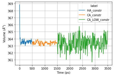
Plot temperature

[35]:

ener_pd_1 = md_sys.sys_history[-2].get_ener(selection_list=['Volume'])
ener_pd_2 = md_sys.sys_history[-1].get_ener(selection_list=['Volume'])
ener_pd_3 = md_sys.get_ener(selection_list=['Volume'])

ener_pd_1['label'] = 'HA_constr'
ener_pd_2['label'] = 'CA_constr'
ener_pd_2['Time (ps)'] = ener_pd_2['Time (ps)'] + ener_pd_1['Time (ps)'].max()
ener_pd_3['label'] = 'CA_LOW_constr'
ener_pd_3['Time (ps)'] = ener_pd_3['Time (ps)'] + ener_pd_2['Time (ps)'].max()

ener_pd = pd.concat([ener_pd_1, ener_pd_2, ener_pd_3])

gmx energy -f data_sim/sys_equi/sys_equi/00_equi_HA/equi_HA_1Y0M.edr -o tmp_edr.xvg
gmx energy -f data_sim/sys_equi/sys_equi/01_equi_CA/equi_CA_1Y0M.edr -o tmp_edr.xvg
gmx energy -f data_sim/sys_equi/sys_equi/02_equi_CA_LOW/equi_CA_LOW_1Y0M.edr -o tmp_edr.xvg

[36]:

ax = sns.lineplot(x="Time (ps)", y="Volume",
                  hue="label",
                  data=ener_pd)

ax.set_ylabel('Volume ($Å^3$)')
plt.grid()

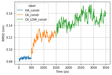
../_images/notebook_00_basic_example_33_0.png

Plot RMSD

[42]:

# Define reference structure for RMSD calculation
ref_sys =  md_sys.sys_history[1]

rmsd_pd_1 = md_sys.sys_history[-2].get_rmsd(['C-alpha', 'Protein'], ref_sys=ref_sys)
rmsd_pd_2 = md_sys.sys_history[-1].get_rmsd(['C-alpha', 'Protein'], ref_sys=ref_sys)
rmsd_pd_3 = md_sys.get_rmsd(['C-alpha', 'Protein'], ref_sys=ref_sys)


rmsd_pd_1['label'] = 'HA_constr'
rmsd_pd_2['label'] = 'CA_constr'
rmsd_pd_2['time'] = rmsd_pd_2['time'] + rmsd_pd_1['time'].max()
rmsd_pd_3['label'] = 'CA_LOW_constr'
rmsd_pd_3['time'] = rmsd_pd_3['time'] + rmsd_pd_2['time'].max()

rmsd_pd = pd.concat([rmsd_pd_1, rmsd_pd_2, rmsd_pd_3])

gmx rms -s data_sim/em/Init_em_1Y0M.tpr -f data_sim/sys_equi/sys_equi/00_equi_HA/equi_HA_1Y0M.xtc -n data_sim/sys_equi/sys_equi/00_equi_HA/equi_HA_1Y0M.ndx -o tmp_rmsd.xvg -fit rot+trans -ng 1 -pbc no
gmx rms -s data_sim/em/Init_em_1Y0M.tpr -f data_sim/sys_equi/sys_equi/01_equi_CA/equi_CA_1Y0M.xtc -n data_sim/sys_equi/sys_equi/01_equi_CA/equi_CA_1Y0M.ndx -o tmp_rmsd.xvg -fit rot+trans -ng 1 -pbc no
gmx rms -s data_sim/em/Init_em_1Y0M.tpr -f data_sim/sys_equi/sys_equi/02_equi_CA_LOW/equi_CA_LOW_1Y0M.xtc -n data_sim/sys_equi/sys_equi/02_equi_CA_LOW/equi_CA_LOW_1Y0M.ndx -o tmp_rmsd.xvg -fit rot+trans -ng 1 -pbc no

[43]:

ax = sns.lineplot(x="time", y="Protein",
                  hue="label",
                  data=rmsd_pd)

ax.set_ylabel('RMSD (nm)')
ax.set_xlabel('Time (ps)')
plt.grid()

../_images/notebook_00_basic_example_36_0.png

Production

[27]:

md_sys.production(out_folder=prod_folder,
                  nsteps=prod_step,
                  dt=dt, vsite=vsite, maxwarn=1)

gmx grompp -f prod_1Y0M.mdp -c ../sys_equi/sys_equi/02_equi_CA_LOW/equi_CA_LOW_1Y0M.gro -r ../sys_equi/sys_equi/02_equi_CA_LOW/equi_CA_LOW_1Y0M.gro -p ../sys_top/1Y0M_water_ion.top -po out_prod_1Y0M.mdp -o prod_1Y0M.tpr -maxwarn 1 -n ../sys_equi/sys_equi/02_equi_CA_LOW/equi_CA_LOW_1Y0M.ndx
gmx mdrun -s prod_1Y0M.tpr -deffnm prod_1Y0M -nt 0 -ntmpi 0 -nsteps -2 -nocopyright

Prepare trajectory

[40]:

# Center trajectory
md_sys.center_mol_box(traj=True)

gmx make_ndx -f data_sim/sys_prod/prod_1Y0M.gro -o data_sim/sys_prod/prod_1Y0M.ndx
gmx trjconv -f data_sim/sys_prod/prod_1Y0M.xtc -o data_sim/sys_prod/prod_1Y0M_compact.xtc -s data_sim/sys_prod/prod_1Y0M.tpr -ur tric -pbc mol -center yes -n data_sim/sys_prod/prod_1Y0M.ndx

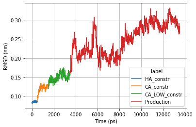
Basic Analysis

[44]:

rmsd_prod_pd = md_sys.get_rmsd(['C-alpha', 'Protein'], ref_sys=ref_sys)
rmsd_prod_pd['label'] = 'Production'

rmsd_prod_pd['time'] = rmsd_prod_pd['time'] + rmsd_pd['time'].max()
rmsd_all_pd = pd.concat([rmsd_pd, rmsd_prod_pd])

gmx rms -s data_sim/em/Init_em_1Y0M.tpr -f data_sim/sys_prod/prod_1Y0M_compact.xtc -n data_sim/sys_prod/prod_1Y0M.ndx -o tmp_rmsd.xvg -fit rot+trans -ng 1 -pbc no

[48]:

ax = sns.lineplot(x="time", y="Protein",
                  hue="label",
                  data=rmsd_all_pd)
ax.set_ylabel('RMSD (nm)')
ax.set_xlabel('Time (ps)')
plt.grid()

../_images/notebook_00_basic_example_43_0.png

Trajectory vizualisation

[58]:

# Align the protein coordinates
md_sys.convert_trj(select='Protein\nSystem\n', fit='rot+trans', pbc='none', skip='10')

gmx trjconv -f data_sim/sys_prod/prod_1Y0M_compact_compact.xtc -o data_sim/sys_prod/prod_1Y0M_compact_compact_compact.xtc -s data_sim/sys_prod/prod_1Y0M.tpr -ur compact -pbc none -fit rot+trans -n data_sim/sys_prod/prod_1Y0M.ndx -skip 10

[70]:

view = md_sys.view_traj()
view.add_representation(repr_type='licorice', selection='protein')
view.center(selection='CA')
view

[4]:

# Unecessary, only need to nglview online:
IFrame(src='../_static/1Y0M_prod_traj.html', width=800, height=300)

[4]:

[ ]: